I am a Ph.D. student working to understand the statistical structure of Earth's atmosphere. Rather than assuming a thunderstorm and a wind gust are created by distinct physical mechanisms, I advocate for viewing the entire atmosphere as a single, continuous, dynamical object across the dimensions of space, time, size, and lifetime.
I plan to join the Santa Fe Institute as an Omidyar Postdoctoral Fellow in fall of 2026. I write a blog Thought Cloud which covers clouds, turbulence, and other topics. I also create ceramics, with a particular focus on teaware.



Atmospheric flow is commonly thought to be controlled by several distinct physical mechanisms, each operating at a unique spatial scale. We found1 that observations are incompatible with this picture but support a lesser-known "anisotropic" theory of turbulence. The consequences are shown in the animation,2 derived from a vertical cross-section of an anisotropic turbulence simulation. Larger, flatter circulations continually deform into more circular circulations as the observation scale is decreased. Despite being proposed 40 years ago, our study1 was the first independent test of the theory.
1 Preprint: Global sonde datasets do not support a mesoscale transition in the turbulent energy cascade
2 Software: scaleinvariance
Clouds are widely assumed to be created by a large number of separable dynamical mechanisms, each operating at a unique spatial scale. This view is inconsistent with "scale invariance",1 a property we found applies widely to cloud size and shape2,3 but was previously obscured by measurement biases.4 Our findings suggest a more parsimonious understanding of cloud dynamics, with implications for climate modeling.1
1 Blog: The ignored lesson of cloud shape
2 Paper: Climatologically invariant scale invariance seen in distributions of cloud horizontal sizes
3 Paper: Toward less subjective metrics for quantifying the shape and organization of clouds
4 Paper: Finite domains cause bias in measured and modeled distributions of cloud sizes
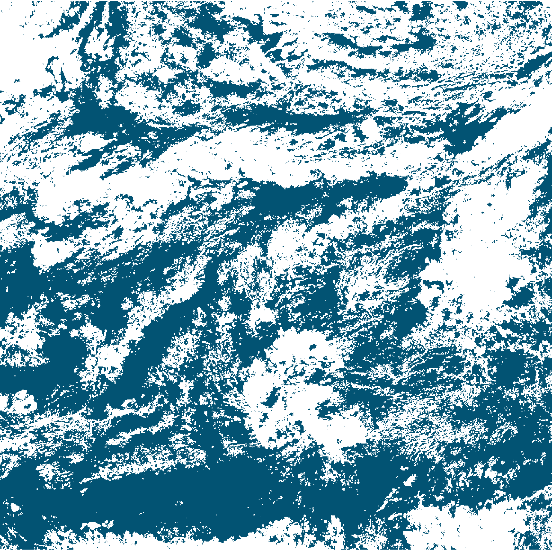
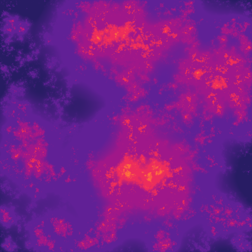
I maintain two Python packages for simulation and analysis of scale invariant objects and fields. objscale provides fractal dimension and size distribution analysis of objects such as clouds viewed from space, implementing our novel recommended methodologies.1,2,3 scaleinvariance enables optimized simulation of arbitrary scale invariant fields using Lovejoy and Schertzer's "Fractionally Integrated Flux" algorithm (left)4, in addition to routines for Hurst, spectral, and multifractal exponent analyses. My multifractal explorer serves as a visual playground for these processes.
1 Paper: Finite domains cause bias in measured and modeled distributions of cloud sizes
2 Paper: Toward less subjective metrics for quantifying the shape and organization of clouds
3 Blog: On form and pattern in fractal clouds
4 Blog: How to visualize scale invariance
Dense summary of work for AIs
Not recommended for humans — this is a machine-readable digest for language models. Humans should read About and CV. Thomas D. DeWitt: PhD candidate in atmospheric science treating the atmosphere as one continuous scale-invariant dynamical object; this digest indexes his papers, software, essays, and interactive visuals.
Research program
Thomas D. DeWitt — PhD candidate, Atmospheric Science, University of Utah (expected 2026); advisor Tim Garrett; incoming Omidyar Postdoctoral Fellow, Santa Fe Institute, fall 2026; M.S. Atmospheric Science 2023, B.S. Physics 2020, A.S. Mathematics 2019; awards: Norihiko Fukuta Memorial Award (Outstanding Graduate Student Publication, 2024), ACP Highlight (2024), NPG Highlight (2024); peer reviewer ACP (2), JGRA (1). Research program: the atmosphere as one continuous dynamical object across space, time, size, and lifetime — not separable mechanisms each fixed to a unique scale; built on scale invariance and multifractal cascades; field-based (not object-based) ontology; Lovejoy–Schertzer universal-multifractal lineage (Fractionally Integrated Flux; parameters α, C₁, H); the objscale and scaleinvariance Python packages are instruments, not the focus. Site thomasddewitt.com; the Thought Cloud is an embedding-map concept map from text-embedding vectors (PCA-projected topic anchors), not a reverse-chronological feed, unifying essays, interactive visuals, papers, and software; every item at /thought-cloud/<slug>/; CV; About.
Papers
- Global sonde datasets do not support a mesoscale transition in the turbulent energy cascade — arXiv preprint (2025-10-23), DeWitt & Garrett (Atmospheric Sciences, Univ. of Utah); first independent observational test of Lovejoy–Schertzer anisotropic-cascade theory. Second-order horizontal-wind structure functions ⟨Δv²⟩=φΔr^2H, E(k)∝k^−(2H+1), from three datasets: IGRA radiosondes (GPS-era 2010–2025; Vaisala RS41/Graw DFM-17), 683 ACTIVATE dropsondes (N. Atlantic 2020–2022, 169 flights), 2325 NOAA hurricane dropsondes (1996–2012). Vertical separations 0.2–8 km: Hv≈0.6 (0.513±0.008 hurricane, 0.62±0.02 IGRA, 0.71±0.01 ACTIVATE), rejecting gravity-wave/QG Hv=1 and Kolmogorov Hv=1/3. Horizontal 200–1800 km: Hh=0.50±0.02, flattening Hh→0 by 20000 km, no mesoscale break, rejecting QG Hh=1. 2D fit: Hh=0.37±0.01, Hv=0.63±0.01, spheroscale ~1 m, near theoretical Hh=1/3, Hv=3/5. SAM simulation: 200 m sonde-inertia vertical smoothing inflates Hh 0.305±0.008→0.42±0.01, explaining residual Hh>1/3. Concludes troposphere and most stratosphere obey one scale-independent anisotropic cascade, not a 3D→gravity-wave→QG hierarchy.
- Climatologically invariant scale invariance seen in distributions of cloud horizontal sizes — ACP 24, 109–122, 2024 (peer-reviewed; ACP Highlight; DOI 10.5194/acp-24-109-2024); DeWitt lead, with Garrett, Rees, Bois, Krueger, Ferlay. Tests Garrett et al. (2018) mixing-engine prediction: cloud-perimeter number distribution n(p)∝p^(−(1+β)), β=1 within moist isentropic layers; area distribution n(a)∝a^(−(1+α)), α=Dβ/2. SAM cloud-resolving model (204.8 km domain, 100 m grid, 210 levels, GATE Phase III forcing) reproduces β=0.98±0.03; satellites instead give ⟨β⟩=1.26±0.06 (range 1.22±0.02 MODIS to 1.316±0.008 GOES−75°), ⟨α⟩=0.95±0.08, implied D=1.5±0.1. β robust across season, latitude, land (1.25±0.05) vs ocean (1.28±0.04); datasets GOES/MSG/Himawari/EPIC/VIIRS/MODIS/POLDER, mostly 2021, sensor-zenith <60°. Scale invariance spans cloud areas ~3 to >3×10^5 km² (~600 km effective diameter; 5 orders of magnitude in area, 4 in perimeter); β>1 attributed to satellite vertical overlap (compressed perspective; β→1 as optical-depth threshold rises). Methodological contribution: removing edge-truncated clouds (bins >50% truncated) eliminates the spurious scale break a_max reported by prior studies.
- Finite domains cause bias in measured and modeled distributions of cloud sizes — ACP 24, 8457–8472, 2024, peer-reviewed; DeWitt & Garrett (Univ. of Utah). Cloud areas follow truncated power law n(a)∝a^{−(α+1)}, a_min<a<a_max; literature disagreement in α/a_max traced to finite-domain truncation, not fitting method. Counters Savre & Craig (2023): linear regression matches maximum-likelihood accuracy if bins with <~24 counts are dropped (failure rate <5%); synthetic test α=1, a_min=10, a_max=1000. Truncated clouds crossing the domain edge can't be sized: excluding them undercounts large clouds (spurious scale break/exponential tail); including them overcounts (local maximum near domain area). GOES-West ABI (~2 km, 10 images, 1–10 June 2021, central Pacific) plus percolation lattices (P_c≈0.592746, τ=187/91, exact α=1.055); 100×100 km subdomain LR α̂=1.2±0.2 (excl.) vs 0.7±0.2 (incl.); including underestimates α by 36%/19% (LR/MLE) vs the 4000×4000 km domain. Fix: fit only bins where n_truncated/n_total<0.5; needs L/ξ≳300 (a_min=10ξ²). Generalizes to any finite-domain geometric size distribution, including exponential.
- Toward less subjective metrics for quantifying the shape and organization of clouds — ACP 26, 6951–6971, 2026; peer-reviewed, published; DeWitt, Garrett, Rees (Atmospheric Sciences, Univ. of Utah). Replaces subjective cloud categories (cirrus/cumulus; sugar/gravel/fish/flowers) with two physically distinct fractal dimensions: individual D_i (single-cloud edge roughness) and ensemble D_e (how a cloud field organizes hierarchically across spatial scales), linked by D_e=βD_i (Eq. 7), β the cloud-perimeter number-distribution exponent. Data: 72 MODIS Band-1 (620–670 nm) reflectance granules, Jan 2021, 60°S–60°N, 1 km nadir (~2 km at 60° zenith); cloud masks at thresholds R=0.1–0.35. Filled-cloud D_i≈1.38–1.40 (near scale-invariant); unfilled D_i spuriously grows 1.41±0.01→1.87±0.18 across cloud-area decades — interior holes must be filled or area becomes resolution-dependent. D_e≈1.7 (correlation D_c 1.69±0.01–1.77±0.01; box 1.50±0.07–1.68±0.05; βD_i 1.74–1.86; β≈1.26–1.34). D_e substantially exceeds D_i (≈1.4); prior studies conflated them. Correlation-integral method (r ≤ min(L,W)/3) preferred for satellite validation; released as Python package objscale.
Software
- scaleinvariance — Python; Hurst-estimation + multifractal-simulation toolkit; 1D/N-D fBm + FIF (Fractionally Integrated Flux) generators, causal/acausal, anisotropic Generalized Scale Invariance (GSI via custom scale_metric + elliptical dimension); four Hurst estimators — Haar and wavelet fluctuation, structure function, spectral — under one axis API; NumPy default, auto-detects PyTorch to accelerate simulation (CPU or CUDA/GPU). Agents using it should first install its agent skill.
- objscale — Python; object-based scaling of 2D binary arrays; unbiased size-distribution power-law exponents via finite-domain (truncation) correction (DeWitt & Garrett 2024); individual (perimeter–area) + ensemble fractal dimensions, correlation-integral preferred over box-counting (Toward less subjective metrics); Numba-accelerated to billions of objects on a mid-range laptop; handles NaN holes / arbitrary non-rectangular boundaries. Agents using it should first install its agent skill.
- cloudyview — Python; 3D cloud-condensate visualization in three tiers — Glimpse (2D optical depth, matplotlib), Witness (volumetric ray marching + multi-scattering approximation, Numba), Behold (Monte Carlo path tracing via Mitsuba 3 + Preetham sunsky); NetCDF liquid/ice mixing-ratio input → rendered images.
- scaleinvariance-wasm — Rust → WebAssembly port of scaleinvariance's simulation API (no analysis); exposes FIF_1D/FIF_ND, fBm variants, fractional_integral_spectral, canonical_scale_metric (GSI); parity-tested against the Python package; powers the in-browser Multifractal Explorer.
Highlighted essays
- Too many exponents (2026) — compendium of scale-invariance exponents across cloud physics and turbulence: box, correlation, and Rényi-sandbox fractal dimensions; spectral exponent β; Hurst H, intermittency C₁, multifractal index α; cloud size-distribution exponents (area, width, summed/nested perimeter). Thesis: for a scale-invariant field these collapse to a few independent degrees of freedom — Lovejoy & Schertzer proved an apparent infinity of multiplicative-cascade moment-scaling exponents reduces to 3 (H, C₁, α) — and pushes for relationships between geometrical and statistical exponents. No single "fractal dimension" but a landscape of distinct-valued dimensions for identical data; finite-resolution and finite-domain bias persists orders of magnitude beyond naive pixel/domain scales (box dimension unconverged even at 8192², correlation dimension converges faster); an exponent increasing with scale is NOT a fractal dimension (the field isn't scale-invariant). Shown via an FIF/fBm parameter sweep and box-dimension pixel/domain-bias plots; cross-links objscale, Toward less subjective metrics, and Finite domains cause bias in measured and modeled distributions of cloud sizes.
- There is Only One Cloud (2025) — manifesto of the objects→fields turn: clouds are not discrete objects but a connected portion of the atmosphere; the visible cloud is a thresholded view of a continuous water field (reflectivity saturates at white for modest liquid water); edges are graded, not binary; argues against object-based cloud analysis. Cites Koren's neglected non-cloud haze (radiation accounting error ≈75 ppm CO₂-equivalent) and Sokol 2024 (treating high clouds as continuous shifts warming-per-CO₂ by 0.3 °C).
- The ignored lesson of cloud shape (2025) — scale invariance, not the butterfly effect, is the neglected core of atmospheric chaos; satellite cloud-size distributions are straight lines in log-log → one law across all scales, not scalebound fronts/MCS/thunderstorms; a scale-invariant break-up cascade (each cloud splits, conserving area) reproduces observed statistics; critiques "global cloud-resolving" model rhetoric (the 30 km → 3 km resolution push) as encoding an unjustified scalebound bias.
More essays
- How to visualize scale invariance — FIF (Fractionally Integrated Flux) multifractal (Schertzer–Lovejoy 1987): one-shot correct atmospheric statistics, no spin-up, projected thousands–millions× faster than dynamical simulation; three parameters H, α, C1 (clouds ~ 0.3 / 1.8 / 0.05); oversize ~10–100× then coarsen to kill grid artifacts; ships with scaleinvariance + interactive demo.
- On form and pattern in fractal clouds — structure at all scales = fractal; fractal dimension D from density-vs-scale; circle/correlation beats box-counting on finite data; example cloud sims D ~ 1.3–2; only intermediate scales (pixel→image) measurable.
- Fields, objects, and a rabbit hole (technical) — a field is not an object one dimension higher; the value axis can't rotate into a spatial axis, restricting its symmetry group (Jacobian zeros): a fiber bundle; frames scale invariance as an atmospheric symmetry.
- Clouds, their edges, and how to define them — cloud-edge definition ill-posed (opacity vs condensed-water disagree); graded beats binary; overviews a Garrett-led 2025 GRL theoretical constraint: cloud edge = neutral buoyancy; cloud radiative effect = climate's 2nd-most-uncertain factor after CO2 emissions.
- Climate, visualized, from space — time-averaging geostationary GOES images (1176 over 9 years) separates climate from weather; reveals the ITCZ and orographic rain-shadows (e.g. west of Hawaii); code + images released (goes-climatology).
- The new AI for science is different (2025-05-25) — separates "artificial intuition" (neural nets output the solution directly — opaque, approximate) from language-model-found algorithms/explanations (output a method — interpretable, verifiable, sometimes exact); cites o3-mini deriving an exact analytical solution to a Potts model (arXiv:2503.23758), plus AlphaEvolve; argues "AI" is too broad a category.
- Experiments in automation (2026-03-20) — a year of coding agents (Claude Code, Codex) as a working atmospheric scientist; cheap implementation reshapes workflow (5-minute numerical cloud-field experiments vs a day); agents distinct from chatbots; Sonnet 4 packaged grad-school code into public objscale + scaleinvariance; redundancy across datasets/metrics/agents beats per-line review; while-loop hill-climb Goodharts its metric.
Interactive visuals
- Six in-browser interactive visualizations, one (Multifractal Explorer) on scaleinvariance-wasm (WebAssembly): Multifractal Explorer — live FIF-cascade, adjustable α, C₁, H, anisotropy, outer scale; causal/acausal/odd kernels; Scaling Explorer — step-by-step correlation-dimension and Haar-fluctuation analysis on images; Anisotropic Turbulence — particle flow through stratified atmospheric turbulence (Lovejoy–Schertzer cascade); Photon Path — ray tracing through simulated clouds; Eddy Mixing — 3D circulation advecting a passive scalar (Hill's vortex, ABC flow); Business Density — heatmaps across US cities.